2022. 1. 21. 01:35ㆍcomputervision/섹션 6. YOLO(You Only Look Once)
Darknet Yolo 사이트에서 coco dataset으로 학습된 inference 모델과 config파일을 이용하여 OpenCV에서 inference모델을 생성해보는 실습이다.
https://pjreddie.com/darknet/yolo/ 에서 weight파일과 config파일을 다운받을 수 있다.
!mkdir ./pretrained
!echo "##### downloading pretrained yolo/tiny-yolo weight file and config file"
!wget -O /content/pretrained/yolov3.weights https://pjreddie.com/media/files/yolov3.weights
!wget -O /content/pretrained/yolov3.cfg https://github.com/pjreddie/darknet/blob/master/cfg/yolov3.cfg?raw=true

!wget -O /content/pretrained/yolov3-tiny.weights https://pjreddie.com/media/files/yolov3-tiny.weights
!wget -O /content/pretrained/yolov3-tiny.cfg https://github.com/pjreddie/darknet/blob/master/cfg/yolov3-tiny.cfg?raw=true

!ls /content/pretrained
pretrained 폴더를 생성후 yolo v3 weight config파일과 tiny yolo v3 weight config파일을 pretrained 폴더에 다운로드 받는다.
import os
import cv2

weights_path = '/content/pretrained/yolov3.weights'
config_path =  '/content/pretrained/yolov3.cfg'

cv_net_yolo = cv2.dnn.readNetFromDarknet(config_path, weights_path)
weight와 config파일의 경로를 설정후 readNetFromDarknet함수를 이용하여 모델을 로딩한다.
이때 config, weight 순서를 주의해야한다.
labels_to_names_seq = {0:'person',1:'bicycle',2:'car',3:'motorbike',4:'aeroplane',5:'bus',6:'train',7:'truck',8:'boat',9:'traffic light',10:'fire hydrant',
                        11:'stop sign',12:'parking meter',13:'bench',14:'bird',15:'cat',16:'dog',17:'horse',18:'sheep',19:'cow',20:'elephant',
                        21:'bear',22:'zebra',23:'giraffe',24:'backpack',25:'umbrella',26:'handbag',27:'tie',28:'suitcase',29:'frisbee',30:'skis',
                        31:'snowboard',32:'sports ball',33:'kite',34:'baseball bat',35:'baseball glove',36:'skateboard',37:'surfboard',38:'tennis racket',39:'bottle',40:'wine glass',
                        41:'cup',42:'fork',43:'knife',44:'spoon',45:'bowl',46:'banana',47:'apple',48:'sandwich',49:'orange',50:'broccoli',
                        51:'carrot',52:'hot dog',53:'pizza',54:'donut',55:'cake',56:'chair',57:'sofa',58:'pottedplant',59:'bed',60:'diningtable',
                        61:'toilet',62:'tvmonitor',63:'laptop',64:'mouse',65:'remote',66:'keyboard',67:'cell phone',68:'microwave',69:'oven',70:'toaster',
                        71:'sink',72:'refrigerator',73:'book',74:'clock',75:'vase',76:'scissors',77:'teddy bear',78:'hair drier',79:'toothbrush' }
이후 coco class id와 class명을 알맞게 mapping시킨다.
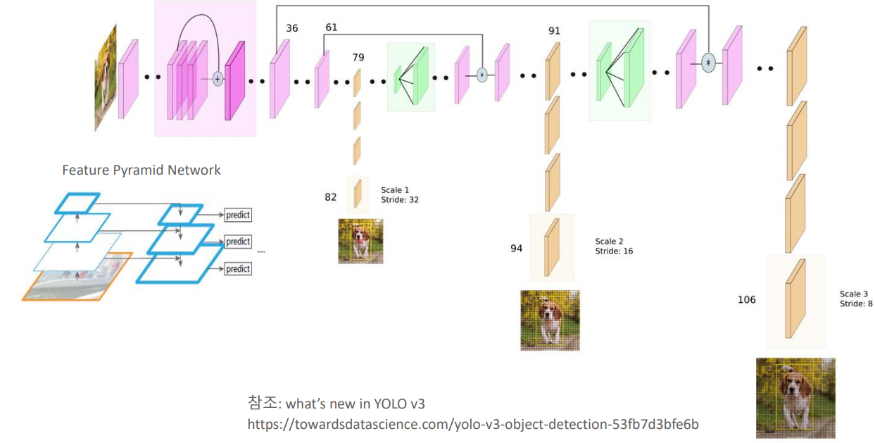
YOLO V3 Network구조에서 위의 그림에서의 82, 94, 106번째 3개의 scale output layer에서 결과 데이터를 추출해야 한다.
layer_names = cv_net_yolo.getLayerNames()
print('final output layer id:', cv_net_yolo.getUnconnectedOutLayers())
print('final output layer name:', [layer_names[i[0] - 1] for i in cv_net_yolo.getUnconnectedOutLayers()])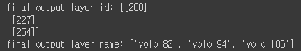
다음과 같은 코드로 위의 3개의 layer를 찾아 낼 수 있다.
#전체 Darknet layer에서 13x13 grid, 26x26, 52x52 grid에서 detect된 Output layer만 filtering
layer_names = cv_net_yolo.getLayerNames()
outlayer_names = [layer_names[i[0] - 1] for i in cv_net_yolo.getUnconnectedOutLayers()]
print('output_layer name:', outlayer_names)

img = cv2.imread('./data/beatles01.jpg')
img_rgb = cv2.cvtColor(img, cv2.COLOR_BGR2RGB)

cv_net_yolo.setInput(cv2.dnn.blobFromImage(img, scalefactor=1/255.0, size=(416, 416), swapRB=True, crop=False))

# Object Detection 수행하여 결과를 cvOut으로 반환
cv_outs = cv_net_yolo.forward(outlayer_names)
print('cv_outs type:', type(cv_outs), 'cv_outs의 내부 원소개수:', len(cv_outs))
print(cv_outs[0].shape, cv_outs[1].shape, cv_outs[2].shape)
classification을 위해서는 위의 3개의 layer에서의 결과값을 반환하여야 한다.
또한 로딩한 모델은 YOLO V3 416*416모델이므로 원본 이미지 배열 사이즈를 416*416으로 reshape해주어야한다.
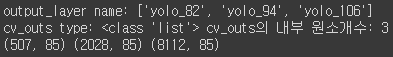
위의 코드의 결과는 왼쪽과 같은데 총 3개의 원하는 layer가 cv_outs의 객체로 들어간 것을 알 수 있고
첫번째, 두번째, 세번째 feature map의 크기가 각각 (13*13*3(3개의 anchor box)), (26*26*3), (52*52*3)으로 잘 출력된 것을 볼 수 있다.
import numpy as np

rows = img.shape[0]
cols = img.shape[1]

conf_threshold = 0.5
nms_threshold = 0.4

# bounding box의 테두리와 caption 글자색 지정
green_color=(0, 255, 0)
red_color=(0, 0, 255)

class_ids = []
confidences = []
boxes = []

# 3개의 개별 output layer별로 Detect된 Object들에 대해서 Detection 정보 추출 및 시각화
for ix, output in enumerate(cv_outs):
    print('output shape:', output.shape)
    # feature map에 있는 anchor 갯수만큼 iteration하면서 Detected 된 Object 추출.(13x13x3, 26x26x3, 52x52x3)
    for jx, detection in enumerate(output):
        # class score는 detetection배열에서 5번째 이후 위치에 있는 값.
        class_scores = detection[5:]
        # class_scores배열에서 가장 높은 값을 가지는 값이 class confidence, 그리고 그때의 위치 인덱스가 class id
        class_id = np.argmax(class_scores)
        confidence = class_scores[class_id]

        # confidence가 지정된 conf_threshold보다 작은 값은 제외
        if confidence > conf_threshold:
            print('ix:', ix, 'jx:', jx, 'class_id', class_id, 'confidence:', confidence)
            # detection은 scale된 좌상단, 우하단 좌표를 반환하는 것이 아니라, detection object의 중심좌표와 너비/높이를 반환
            # 원본 이미지에 맞게 scale 적용 및 좌상단, 우하단 좌표 계산
            center_x = int(detection[0] * cols)
            center_y = int(detection[1] * rows)
            width = int(detection[2] * cols)
            height = int(detection[3] * rows)
            left = int(center_x - width / 2)
            top = int(center_y - height / 2)
            # 3개의 개별 output layer별로 Detect된 Object들에 대한 class id, confidence, 좌표정보를 모두 수집
            class_ids.append(class_id)
            confidences.append(float(confidence))
            boxes.append([left, top, width, height])
3개의 scale output layer에서 object detection 정보(class_id, confidence score, bbox)를 추출한다.
추출된 정보는 class_ids, confidences, boxes 배열에 저장된다.
conf_threshold = 0.5
nms_threshold = 0.4
idxs = cv2.dnn.NMSBoxes(boxes, confidences, conf_threshold, nms_threshold)
이후 confidence_threshold와 nms_threshold의 값을 설정후 NMS를 이용하여 output layer에서 detected된 object의 겹치는 bbox를 제외시킨다.
import matplotlib.pyplot as plt
draw_img = img.copy()
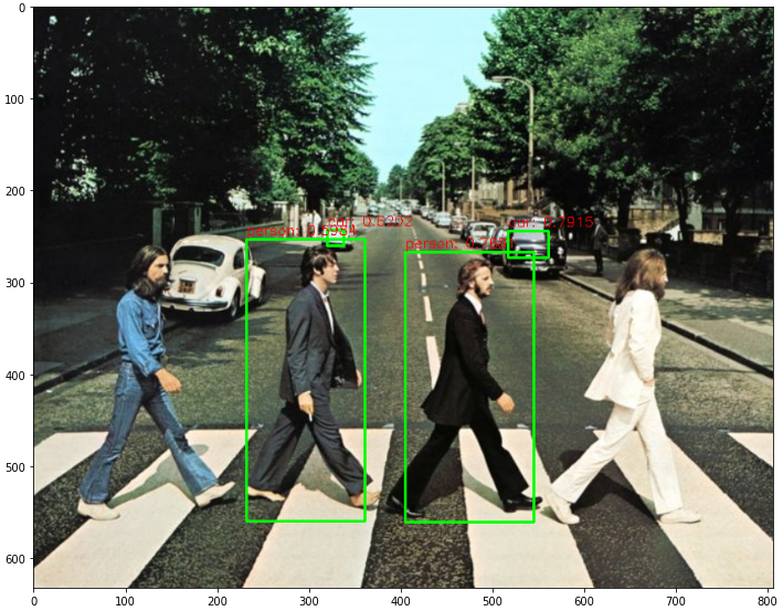
# NMS로 최종 filtering된 idxs를 이용하여 boxes, classes, confidences에서 해당하는 Object정보를 추출하고 시각화.
if len(idxs) > 0:
for i in idxs.flatten():
box = boxes[i]
left = box[0]
top = box[1]
width = box[2]
height = box[3]
# labels_to_names 딕셔너리로 class_id값을 클래스명으로 변경. opencv에서는 class_id + 1로 매핑해야함.
caption = "{}: {:.4f}".format(labels_to_names_seq[class_ids[i]], confidences[i])
#cv2.rectangle()은 인자로 들어온 draw_img에 사각형을 그림. 위치 인자는 반드시 정수형.
cv2.rectangle(draw_img, (int(left), int(top)), (int(left+width), int(top+height)), color=green_color, thickness=2)
cv2.putText(draw_img, caption, (int(left), int(top - 5)), cv2.FONT_HERSHEY_SIMPLEX, 0.5, red_color, 1)
print(caption)
img_rgb = cv2.cvtColor(draw_img, cv2.COLOR_BGR2RGB)
plt.figure(figsize=(12, 12))
plt.imshow(img_rgb)NMS로 최종 filtering된 idxs 정보를 이용하여 class_ids, confidences, boxes 배열에서 해당하는 object정보를 추출하여 시각화한다.
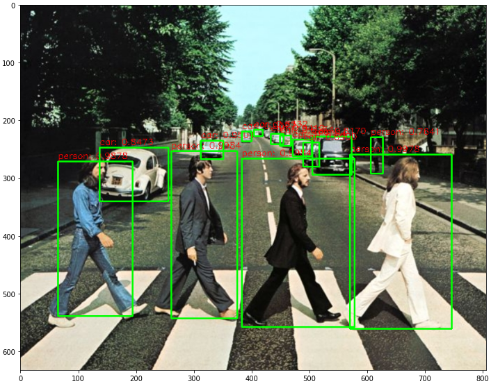
YOLO V3의 특성상 CPU에서는 inference 속도가 원하는 만큼의 성능을 내기가 어려웠다. CPU환경에서는 YOLO의 사용이 크게 효과를 내지 못하는 것 같다.
tiny yolo에서는 CPU환경에서도 위의 yolo v3보다 빠른 성능을 보여주었다. 하지만 confidence_threshold의 값을 0.5정도로 주었을때
다음과 같은 성능을 보여주었다. CPU를 사용해서 학습시 inference time 시간에서는 tiny yolo의 사용이 맞지만 예측 성능이 좋지 못하였다.
'computervision > 섹션 6. YOLO(You Only Look Once)' 카테고리의 다른 글
| CVAT 사용해보기 (0) | 2022.01.27 |
|---|---|
| Ultralytics Yolo 실습(Oxford pet dataset) (0) | 2022.01.25 |
| YOLO(V3) 이해 (0) | 2022.01.20 |
| YOLO(V2) 이해 (0) | 2022.01.20 |
| YOLO(V1) 이해 (0) | 2022.01.20 |